How can we find all rational points on an elliptic curve?

Known

1. The Elliptic Curve(ECC) equation: $y^2 = x^3 - 2x$
2. A point on the ECC: $P_0 : (x_0, y_0)$

A Better Defined Problem

Instead of trying to find all rational points on an ECC outright, how about we try to solve the following problem which appears to be better defined and might also give us the insight needed to find all rational points.

Given a single point $P_0 : (x_0, y_0)$ on an elliptic curve, can we derive an explicit formula in terms of $x_0$ and $y_0$ for another find another point $P_1 : (x_1, y_1)$ on the ECC?

Our ECC in Sympy

# setup
%matplotlib inline
import matplotlib.pyplot as plt
from sympy import *
x, y, x_0, y_0 = symbols('x, y, x_0, y_0')

# our ECC equation re-arranged
ECC = x**3 - 2*x - y**2
Eq(0, ECC)

$\displaystyle 0 = x^{3} - 2 x - y^{2}$

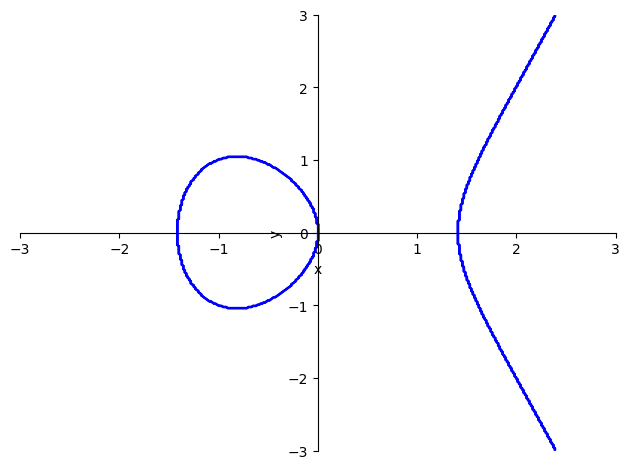
Visualize ECC

square_bound = (-3, 3)
ECC_plot = plot_implicit(
    Eq(0, ECC), (x, *square_bound), (y, *square_bound),
    adaptive=False, points=400);

Begin With a Tangent Line

One way to find another point on the ECC in terms of $(x_0, y_0)$ is to construct a line tangent with $P_0$ that also intersects with the ECC at a point other than $P_0$.

# get slope at P_0
dydx          = idiff(ECC, y, x)
tangent_slope = dydx.subs({x : x_0, y : y_0})
tangent_slope

$\displaystyle \frac{3 x_{0}^{2} - 2}{2 y_{0}}$

# form line tangent to P_0 using slope at P_0
tangent_l = tangent_slope*(x - x_0) + y_0 - y
Eq(0, tangent_l)

$\displaystyle 0 = - y + y_{0} + \frac{\left(x - x_{0}\right) \left(3 x_{0}^{2} - 2\right)}{2 y_{0}}$

Rewrite Tangent Line

We rewrite our tangent line by making use of the fact that: $y_0^2 = x_0^3 - 2x_0 \rightarrow y_0 = \sqrt {x_0^3 -2x_0}$

tangent_l = tangent_l.subs(y_0, sqrt(x_0**3 - 2*x_0)) + y
Eq(y, tangent_l)

$\displaystyle y = \frac{\left(x - x_{0}\right) \left(3 x_{0}^{2} - 2\right)}{2 \sqrt{x_{0}^{3} - 2 x_{0}}} + \sqrt{x_{0}^{3} - 2 x_{0}}$

Visualize Tangent line at

$x_0 = -1$

# this is the tangent line equation when x_0 = -1
tangent_l_eval = tangent_l.subs(x_0, -1)
Eq(y, tangent_l_eval)

$\displaystyle y = \frac{x}{2} + \frac{3}{2}$

tangent_l_eval_plot = plot_implicit(
                        Eq(y, tangent_l_eval),
                        (x, *square_bound), (y, *square_bound),
                        line_color='red',
                        show = False,
                        adaptive=False, points=400);

tangent_l_eval_plot.extend(ECC_plot)
tangent_l_eval_plot.show()

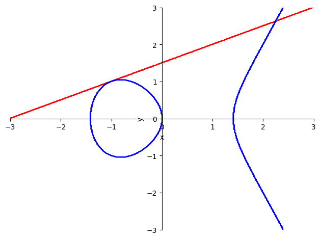
As you can see above, the tangent line intersects the ECC twice. The tangent line is tangent at $P_0 = (-1, 1)$.

We're now trying to find an equation for the second intesection that we see in the upper right quadrant of the graph above in terms of $P_0$.

Intersection

The intersection of the red line and blue line can be solved for by substituting our tangent line into the ECC.

intersection = ECC.subs(y, tangent_l)
intersection

$\displaystyle x^{3} - 2 x - \left(\frac{\left(x - x_{0}\right) \left(3 x_{0}^{2} - 2\right)}{2 \sqrt{x_{0}^{3} - 2 x_{0}}} + \sqrt{x_{0}^{3} - 2 x_{0}}\right)^{2}$

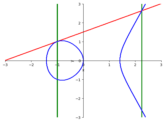
Let's visualize the x-component of the intersections real quick for $x_0 = -1$.

intersection_plot = plot_implicit(
                        Eq(0, intersection.subs(x_0, -1)),
                        (x, *square_bound), (y, *square_bound),
                        line_color='green',
                        show = False,
                        adaptive=False, points=400)
intersection_plot.extend(tangent_l_eval_plot)
intersection_plot.show()

Is there a way we can express the x-coordinate of the of the green line to the right in terms of x-component of the green line to the left?

Yes! This is because the x-coordinate to the left is defined already as $x_0$.

Finding $P_1$

By solving analytically for the intersection of our tangent line with the ECC, we can find $P_{1x}$

Lets refer to the intersection as $f(x)$ such that $f(x) = f_1(x) + f_2(x) + f_3(x) + f_4(x)$.

f_x = collect(expand(intersection), x); f_x

$\displaystyle x^{3} + x^{2} \left(- \frac{9 x_{0}^{4}}{4 x_{0}^{3} - 8 x_{0}} + \frac{12 x_{0}^{2}}{4 x_{0}^{3} - 8 x_{0}} - \frac{4}{4 x_{0}^{3} - 8 x_{0}}\right) + x \left(\frac{18 x_{0}^{5}}{4 x_{0}^{3} - 8 x_{0}} - \frac{24 x_{0}^{3}}{4 x_{0}^{3} - 8 x_{0}} - 3 x_{0}^{2} + \frac{8 x_{0}}{4 x_{0}^{3} - 8 x_{0}}\right) - \frac{9 x_{0}^{6}}{4 x_{0}^{3} - 8 x_{0}} + \frac{12 x_{0}^{4}}{4 x_{0}^{3} - 8 x_{0}} + 2 x_{0}^{3} - \frac{4 x_{0}^{2}}{4 x_{0}^{3} - 8 x_{0}}$

Defining $f_1$ through $f_4 \ldots$

divisor = 4*x_0**3 - 8*x_0; divisor

$\displaystyle 4 x_{0}^{3} - 8 x_{0}$

f1 = x**3; f1

$\displaystyle x^{3}$

f2 = x**2*( (-9*x_0**4)/(divisor) + (12*x_0**2)/(divisor) - (4)/(divisor)); f2

$\displaystyle x^{2} \left(- \frac{9 x_{0}^{4}}{4 x_{0}^{3} - 8 x_{0}} + \frac{12 x_{0}^{2}}{4 x_{0}^{3} - 8 x_{0}} - \frac{4}{4 x_{0}^{3} - 8 x_{0}}\right)$

f3 = x*((18*x_0**5)/(divisor) - (24*x_0**3)/(divisor) - 3*x_0**2 + (8*x_0)/(divisor)); f3

$\displaystyle x \left(\frac{18 x_{0}^{5}}{4 x_{0}^{3} - 8 x_{0}} - \frac{24 x_{0}^{3}}{4 x_{0}^{3} - 8 x_{0}} - 3 x_{0}^{2} + \frac{8 x_{0}}{4 x_{0}^{3} - 8 x_{0}}\right)$

f4 = -(9*x_0**6)/(divisor) + (12*x_0**4)/(divisor) + 2*x_0**3 - (4*x_0**2)/(divisor); f4

$\displaystyle - \frac{9 x_{0}^{6}}{4 x_{0}^{3} - 8 x_{0}} + \frac{12 x_{0}^{4}}{4 x_{0}^{3} - 8 x_{0}} + 2 x_{0}^{3} - \frac{4 x_{0}^{2}}{4 x_{0}^{3} - 8 x_{0}}$

Sanity check.

f_x == f1 + f2 + f3 + f4

True

Let's factor $f_2$, $f_3$, and $f_4 \ldots$

f2_new = -x**2*(3*x_0**2 - 2)**2/divisor; f2_new

$\displaystyle - \frac{x^{2} \left(3 x_{0}^{2} - 2\right)^{2}}{4 x_{0}^{3} - 8 x_{0}}$

f3_new = (2*x*x_0*(3*x_0**2 - 2)**2)/divisor - 3*x*x_0**2; f3_new

$\displaystyle - 3 x x_{0}^{2} + \frac{2 x x_{0} \left(3 x_{0}^{2} - 2\right)^{2}}{4 x_{0}^{3} - 8 x_{0}}$

f4_new = (-x_0**2*(3*x_0**2 - 2)**2)/divisor + 2*x_0**3; f4_new

$\displaystyle 2 x_{0}^{3} - \frac{x_{0}^{2} \left(3 x_{0}^{2} - 2\right)^{2}}{4 x_{0}^{3} - 8 x_{0}}$

More sanity checks.

assert expand(f2) == expand(f2_new)
assert expand(f3) == expand(f3_new)
assert expand(f4) == expand(f4_new)

Let's consolidate some terms...

f1 + f2_new + f3_new + f4_new

$\displaystyle x^{3} - \frac{x^{2} \left(3 x_{0}^{2} - 2\right)^{2}}{4 x_{0}^{3} - 8 x_{0}} - 3 x x_{0}^{2} + \frac{2 x x_{0} \left(3 x_{0}^{2} - 2\right)^{2}}{4 x_{0}^{3} - 8 x_{0}} + 2 x_{0}^{3} - \frac{x_{0}^{2} \left(3 x_{0}^{2} - 2\right)^{2}}{4 x_{0}^{3} - 8 x_{0}}$

consolidate = x**3 - 3*x*x_0**2 + 2*x_0**3 + (-x**2 + 2*x*x_0 + -x_0**2)*((3*x_0**2 - 2)**2)/divisor
#sanity check
assert expand(consolidate) == expand(f_x)
consolidate

$\displaystyle x^{3} - 3 x x_{0}^{2} + 2 x_{0}^{3} + \frac{\left(3 x_{0}^{2} - 2\right)^{2} \left(- x^{2} + 2 x x_{0} - x_{0}^{2}\right)}{4 x_{0}^{3} - 8 x_{0}}$

some more factoring...

consolidate = (x - x_0)**2*(x + 2*x_0) + (-x**2 + 2*x*x_0 + -x_0**2)*((3*x_0**2 - 2)**2)/divisor
# sanity check
assert expand(consolidate) == expand(f_x)
consolidate

$\displaystyle \left(x - x_{0}\right)^{2} \left(x + 2 x_{0}\right) + \frac{\left(3 x_{0}^{2} - 2\right)^{2} \left(- x^{2} + 2 x x_{0} - x_{0}^{2}\right)}{4 x_{0}^{3} - 8 x_{0}}$

even more factoring

consolidate = (x - x_0)**2*(x + 2*x_0) - (x - x_0)**2*((3*x_0**2 - 2)**2)/divisor
# sanity check
assert expand(consolidate) == expand(f_x)
consolidate

$\displaystyle \left(x - x_{0}\right)^{2} \left(x + 2 x_{0}\right) - \frac{\left(x - x_{0}\right)^{2} \left(3 x_{0}^{2} - 2\right)^{2}}{4 x_{0}^{3} - 8 x_{0}}$

This expression is actually the rhs of the following equation.

lhs, rhs = 0, consolidate
Eq(lhs, rhs)

$\displaystyle 0 = \left(x - x_{0}\right)^{2} \left(x + 2 x_{0}\right) - \frac{\left(x - x_{0}\right)^{2} \left(3 x_{0}^{2} - 2\right)^{2}}{4 x_{0}^{3} - 8 x_{0}}$

Multiply both sides by $(x - x_0)^2$

rhs = (x + 2*x_0) - ((3*x_0**2 - 2)**2)/divisor
Eq(0, rhs)

$\displaystyle 0 = x + 2 x_{0} - \frac{\left(3 x_{0}^{2} - 2\right)^{2}}{4 x_{0}^{3} - 8 x_{0}}$

Add fraction to both sides.

rhs = rhs + ((3*x_0**2 - 2)**2)/divisor
lhs = lhs + ((3*x_0**2 - 2)**2)/divisor
Eq(lhs, rhs)

$\displaystyle \frac{\left(3 x_{0}^{2} - 2\right)^{2}}{4 x_{0}^{3} - 8 x_{0}} = x + 2 x_{0}$

Subtract $2x_0$ from both sides.

rhs = rhs - 2*x_0
lhs = lhs - 2*x_0
Eq(lhs, rhs)

$\displaystyle - 2 x_{0} + \frac{\left(3 x_{0}^{2} - 2\right)^{2}}{4 x_{0}^{3} - 8 x_{0}} = x$

Final Answer

sol = simplify(lhs)
Eq(sol, rhs)

$\displaystyle \frac{\frac{x_{0}^{4}}{4} + x_{0}^{2} + 1}{x_{0} \left(x_{0}^{2} - 2\right)} = x$

Some remarks

The solution we found above only is a function of $x_0$ that only consists of fractions and integer powers. So if $x_0$ is rational, the solution we found above is rational.

Once we know one rational point, we can find infintely more. In fact, let's write a function that does just that.

def next_rational_point(x_coord):
    next_x =sol.subs(x_0, x_coord)
    y = sqrt(next_x**3 - 2*next_x)
    return (next_x, y)

res = next_rational_point(-1)
print(res)
next_rational_point(res[0])

(9/4, 21/8)





(12769/7056, 900271/592704)

These results align well the the content here, although the analytical solution presented for finding subsequent rational points seems to differ in sign. I wonder if its a typo as the above numerical evaluations seem to be identical to the one presented in the link above.